Whether ‘tis nobler to stay in or go out
At a certain age many of us wrestle with the decision of whether or not to go out, whether to go to a specific place, and whether it was worth it given the options. This is usually during a youthful period and as such is characterized by abundant energy, the typical enthusiasm, and general excitement. We are having fun and we want more of it, routinely. When we believe that we have missed out it counts against us. We feel this “bad” decision and we punish ourselves doubly by chastising ourselves. With time (read: as we age) we begin to weigh more heavily the effort required to go out and we increasingly compare it against the not so many spectacular nights of the past. Sometimes the places we go to are too packed, occasionally dead, or just lack some vital mix that made the first 15 visits appealing (really the first couple, followed by a dozen extra trips to the well in the hopes of keeping the good times flowing).
We come to our own decisions on how much to discount the night out and in our own sweet time. However, we are not wholly unique in our appraisals, going through this process at roughly the same time as our peers. We are unavoidably influenced by others, by the often felt pressure to conform to the group and by the environment we encounter as a result of multiple individual decisions. The behavior of others affect the environment we encounter, which impact our actions, which in turn influences others, which sways these others, and back again. What we have is a complex system by virtue of interaction, impact, and feedback. Interestingly, these various and disparate decisions can often times lead to global emergent behavior that appears quite regular on the surface even while every molecule is bubbling up underneath.
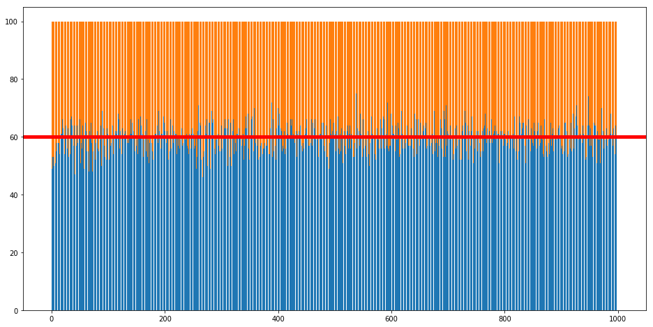
A complex adaptive system portrayed as a going/not going to a bar decision is described in Neil Johnson’s Simply Complexity. The set up as outlined is quite simple: there are 100 people, each of whom has a probability of going out to a local bar; the upper limit (capacity) for comfortable patrons is 60; if someone chooses to go to the bar and there are 60 or fewer patrons it is considered a good decision, if the number creeps above and the bar gets packed the better decision would have been to stay home and those that made just such a decision are the winners on that given night; the “correct“ decision is known that very night, so each patron has an idea of how they fared. Additionally, there is a group memory of a certain number of past nights and their correct decisions. Lastly, if too many bad decisions are made the patrons reevaluate their going out preferences and readjust in the direction that appears most relevant given this public recent memory.
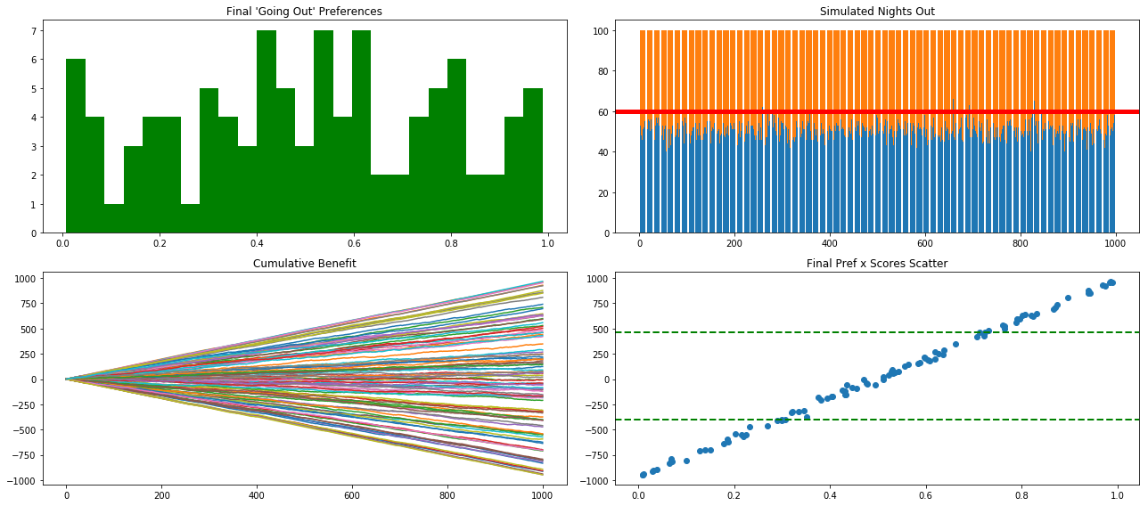
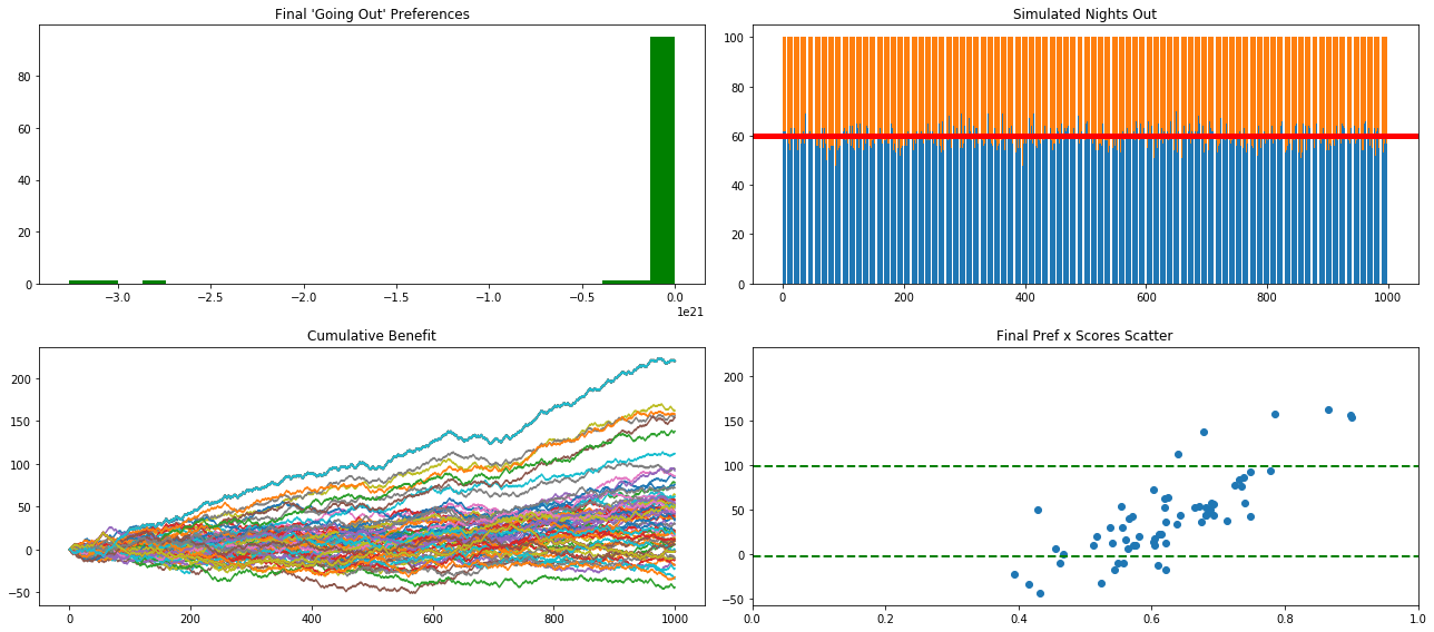
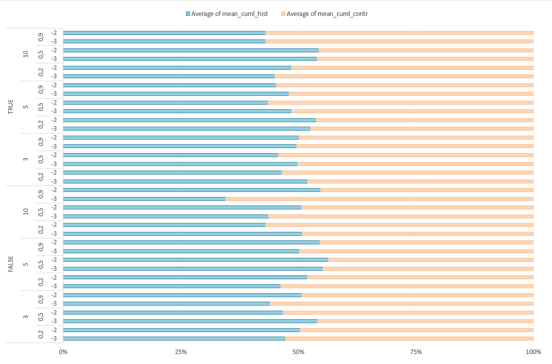
To provide a flavor of the changes taking place when patrons/agents update their preferences compare the above charts with those just below. In the first we left the agents to their original going out preferences and provided utitily scores based on outcomes. As you can see in the bottom left quadrant there is a linear and predictable disparity in outcomes. Contrast this to a collection of patrons who are actively vying for elbow room at the bar and we get a much more interesting result.
In search of an anti-crowd
Despite not being able to reproduce the divergent peaks of crowd and anti-crowd across the probability scale, akin to a double-hump camel, I was able to see similar clusterings occurring regardless of settings; these were typically one large group between .4 and .6 with a long tail toward the higher ranges, .9. I took the added step of capturing the mean and IQR score to get an idea of what worked best overall as a going out policy. This was done by running the simulation (fancy word for function with several for-loops) with different settings on several thresholds, the number of recent nights to keep in memory, and learning rate (or how aggressively to update preferences give an unhappy results and knowing what you should have done). These settings were implemented in thousand (bar) run steps and then again 100 times each. This allowed me to take advantage of the central limit theorem and plot with greater confidence the outcomes over the long run.
Behind a velvet rope of ignorance
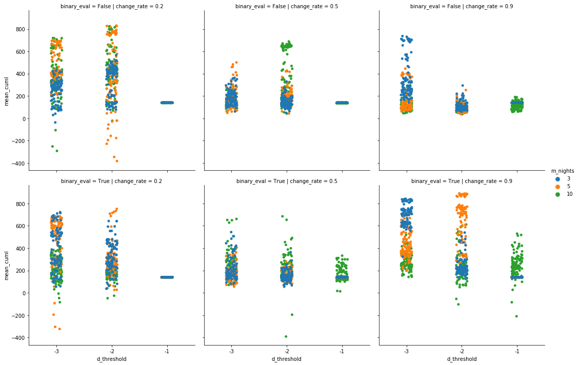
Of the numerous settings and runs referenced the below scatter boxplots were generated. The first group of six shows results when there are no contrarians in the population. This means that the historical outcomes in memory are a good indicator of the future and that those who are unhappy with their performance will update their preferences of either going out or staying in-line with the recent past. Each group of charts has two rows. The top row is binary evaluation set to False, the bottom row to True. “Binary evaluation” has to do with how agents considered the recent night results in memory. If binary agents would update their preferences closer to either 0 or 1, depending on what the historical indication was. Binary False meant updates were made directionally toward the past’s ratio of best decisions (i.e., closer to 70% if the last ten results suggested going out seven times and staying in three).
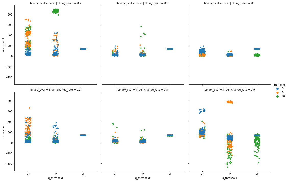
The columns of the scatter boxplots represent different learning rates, how aggresively to update toward the historical (or anti-historical) results. The closer to zero the larger the step and the more dramatic the change in preference. The x-axis indicates the three thresholds patrons were willing to fall behind overall before reevaluating. Both correct and incorrect choices counted as one point. The y-axis indicates the mean ending score1 for each setting/run, with the different color dots suggesting the number of past nights kept in (the public) mind.
Wanting to get an idea of what policy generally turned out the best (average) result the top quartile of utility scores (y-axis) was identified (~192 points). Settings and corresponding results were labeled as either high or low bases on this cutoff. Two ML approaches were run to get an idea of what was important.2 The first was a logistical regression model.
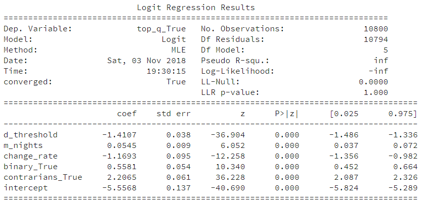
By reviewing the coefficients we can summarize with the following:
- increases your shot of a good time:
- the more nights taken into consideration
- updating preferences as binary decision: go / don’t go
- BIG ONE: having contrarians in the population
- decreases shot at good times:
- making threshold too tight/close to zero
- changing preferences too aggresively
Rules of distraction
A decision tree was also run for good measure and the probabilities of falling into one category or another were used to create a decision matrix/heatmap:3
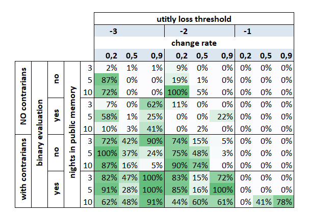
Channeling my inner Michael Pollan: check for contrarians, update preferences toward simple more/less, take as many recent nights into consideration as possible.
Lastly, if you believe the historian/contrarian split is about 50/50, which it was close to in these runs, give the contrarian view a slight edge. Do yourself a favor and buck tradition. Ever so slightly.
Notes
1 Mean was used over median because it better captured the overall/longterm outcomes. While in the original setup patrons have their utility score reset to 0 each time they update their preferences (due to poor performance) and by default have a floor on how low they can score, I retained a running/cummulative tally to get an idea how much beyond (below?) the threshold they were scoring. ↩
2 The goal was backward looking not prediction/generalizability, so you will not see any cross validation. ↩
3 Let the record show I CANNOT spell utility. ↩