analysis template source: https://github.com/data-skeptic/CausalImpact/blob/master/Notebook/GunControl.ipynb
library(CausalImpact)
library("pageviews")
library("assertthat")
Loading required package: bsts
Loading required package: BoomSpikeSlab
Loading required package: Boom
Loading required package: MASS

Attaching package: 'Boom'

The following object is masked from 'package:stats':

    rWishart

Loading required package: zoo

Attaching package: 'zoo'

The following objects are masked from 'package:base':

    as.Date, as.Date.numeric

Loading required package: xts
Taps Fish House
trend.taps <- read.csv('timelines_causalimpact/multiTimeline (64).csv', sep = ',',
                        stringsAsFactors = FALSE)

sapply(trend.taps, typeof)
sapply(trend.taps, class)

colnames(trend.taps)
head(trend.taps)
<dl class=dl-horizontal> <dt>Day</dt> <dd>‘character’</dd> <dt>taps.fish.house.and.brewery</dt> <dd>‘integer’</dd> <dt>Downtown.Joes.Brewery.and.Restaurant</dt> <dd>‘integer’</dd> <dt>Taplands.Brewery</dt> <dd>‘integer’</dd> <dt>Woods.Bar…Brewery</dt> <dd>‘integer’</dd> <dt>Miners.Alley.Brewing.Company</dt> <dd>‘integer’</dd> </dl>
<dl class=dl-horizontal> <dt>Day</dt> <dd>‘character’</dd> <dt>taps.fish.house.and.brewery</dt> <dd>‘integer’</dd> <dt>Downtown.Joes.Brewery.and.Restaurant</dt> <dd>‘integer’</dd> <dt>Taplands.Brewery</dt> <dd>‘integer’</dd> <dt>Woods.Bar…Brewery</dt> <dd>‘integer’</dd> <dt>Miners.Alley.Brewing.Company</dt> <dd>‘integer’</dd> </dl>
<ol class=list-inline> <li>‘Day’</li> <li>‘taps.fish.house.and.brewery’</li> <li>‘Downtown.Joes.Brewery.and.Restaurant’</li> <li>‘Taplands.Brewery’</li> <li>‘Woods.Bar…Brewery’</li> <li>‘Miners.Alley.Brewing.Company’</li> </ol>
| Day | taps.fish.house.and.brewery | Downtown.Joes.Brewery.and.Restaurant | Taplands.Brewery | Woods.Bar...Brewery | Miners.Alley.Brewing.Company |
|---|---|---|---|---|---|
| 2016-07-01 | 0 | 0 | 0 | 0 | 0 |
| 2016-07-02 | 0 | 0 | 0 | 0 | 0 |
| 2016-07-03 | 0 | 0 | 0 | 0 | 0 |
| 2016-07-04 | 0 | 0 | 0 | 0 | 0 |
| 2016-07-05 | 0 | 0 | 0 | 0 | 0 |
| 2016-07-06 | 0 | 0 | 0 | 0 | 0 |
y_trend <- trend.taps[2]
x1_trend <- trend.taps[3]
x2_trend <- trend.taps[4]
x3_trend <- trend.taps[5]
x4_trend <- trend.taps[6]
time.points <- seq.Date(as.Date("2016-07-01"), by = 1, length.out = nrow(y_trend))
data_trend <- zoo(cbind(y_trend, x1_trend, x2_trend, x3_trend, x4_trend), time.points)
colnames(data_trend) <- c("y", "x1", "x2", "x3", "x4")
head(data_trend)
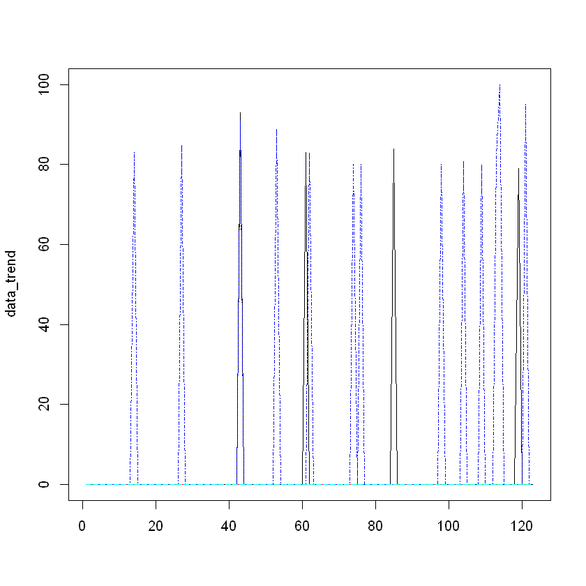
matplot(data_trend, type = "l")
           y x1 x2 x3 x4
2016-07-01 0  0  0  0  0
2016-07-02 0  0  0  0  0
2016-07-03 0  0  0  0  0
2016-07-04 0  0  0  0  0
2016-07-05 0  0  0  0  0
2016-07-06 0  0  0  0  0
pre.period <- as.Date(c("2016-07-01", "2016-10-05"))
post.period <- as.Date(c("2016-10-09", "2016-10-31"))

impact <- CausalImpact(data_trend, pre.period, post.period)
options(warn=-1) # suppresses warnings form geom_path about missing row values
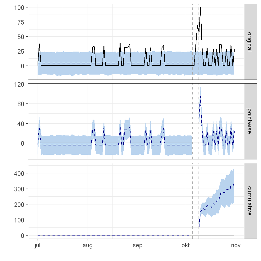
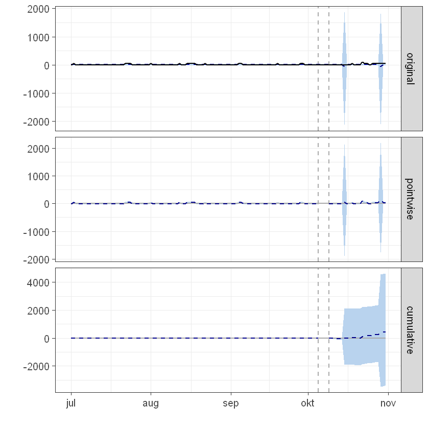
plot(impact)
options(warn=0) # restore warnings
summary: taps.fish.house.and.brewery
summary(impact)

summary(impact,"report")

impact$summary
Posterior inference {CausalImpact}

                         Average         Cumulative
Actual                   3.4             79.0
Prediction (s.d.)        3.4 (3.3)       79.3 (74.9)
95% CI                   [-3, 9.6]       [-69, 220.5]

Absolute effect (s.d.)   -0.013 (3.3)    -0.301 (74.9)
95% CI                   [-6.2, 6.4]     [-141.5, 148.2]

Relative effect (s.d.)   -0.38% (94%)    -0.38% (94%)
95% CI                   [-178%, 187%]   [-178%, 187%]

Posterior tail-area probability p:   0.491
Posterior prob. of a causal effect:  51%

For more details, type: summary(impact, "report")

Analysis report {CausalImpact}


During the post-intervention period, the response variable had an average value of approx. 3.43. In the absence of an intervention, we would have expected an average response of 3.45. The 95% interval of this counterfactual prediction is [-3.01, 9.59]. Subtracting this prediction from the observed response yields an estimate of the causal effect the intervention had on the response variable. This effect is -0.013 with a 95% interval of [-6.15, 6.44]. For a discussion of the significance of this effect, see below.

Summing up the individual data points during the post-intervention period (which can only sometimes be meaningfully interpreted), the response variable had an overall value of 79.00. Had the intervention not taken place, we would have expected a sum of 79.30. The 95% interval of this prediction is [-69.22, 220.51].

The above results are given in terms of absolute numbers. In relative terms, the response variable showed a decrease of-0%. The 95% interval of this percentage is [-178%, +187%].

This means that, although it may look as though the intervention has exerted a negative effect on the response variable when considering the intervention period as a whole, this effect is not statistically significant, and so cannot be meaningfully interpreted. The apparent effect could be the result of random fluctuations that are unrelated to the intervention. This is often the case when the intervention period is very long and includes much of the time when the effect has already worn off. It can also be the case when the intervention period is too short to distinguish the signal from the noise. Finally, failing to find a significant effect can happen when there are not enough control variables or when these variables do not correlate well with the response variable during the learning period.

The probability of obtaining this effect by chance is p = 0.491. This means the effect may be spurious and would generally not be considered statistically significant.
| Actual | Pred | Pred.lower | Pred.upper | Pred.sd | AbsEffect | AbsEffect.lower | AbsEffect.upper | AbsEffect.sd | RelEffect | RelEffect.lower | RelEffect.upper | RelEffect.sd | alpha | p | |
|---|---|---|---|---|---|---|---|---|---|---|---|---|---|---|---|
| Average | 3.434783 | 3.447871 | -3.009474 | 9.587261 | 3.257756 | -0.01308792 | -6.152478 | 6.444257 | 3.257756 | -0.003795942 | -1.784428 | 1.869054 | 0.9448603 | 0.05 | 0.491 |
| Cumulative | 79.000000 | 79.301022 | -69.217910 | 220.506996 | 74.928391 | -0.30102208 | -141.506996 | 148.217910 | 74.928391 | -0.003795942 | -1.784428 | 1.869054 | 0.9448603 | 0.05 | 0.491 |
12Degree
trend.12degree <- read.csv('timelines_causalimpact/multiTimeline (65).csv', sep = ',',
stringsAsFactors = FALSE)
sapply(trend.12degree, typeof)
sapply(trend.12degree, class)
colnames(trend.12degree)
head(trend.12degree)
################
y_trend <- trend.12degree[2]
x1_trend <- trend.12degree[3]
x2_trend <- trend.12degree[4]
x3_trend <- trend.12degree[5]
x4_trend <- trend.12degree[6]
time.points <- seq.Date(as.Date("2016-07-01"), by = 1, length.out = nrow(y_trend))
data_trend <- zoo(cbind(y_trend, x1_trend, x2_trend, x3_trend, x4_trend), time.points)
colnames(data_trend) <- c("y", "x1", "x2", "x3", "x4")
head(data_trend)
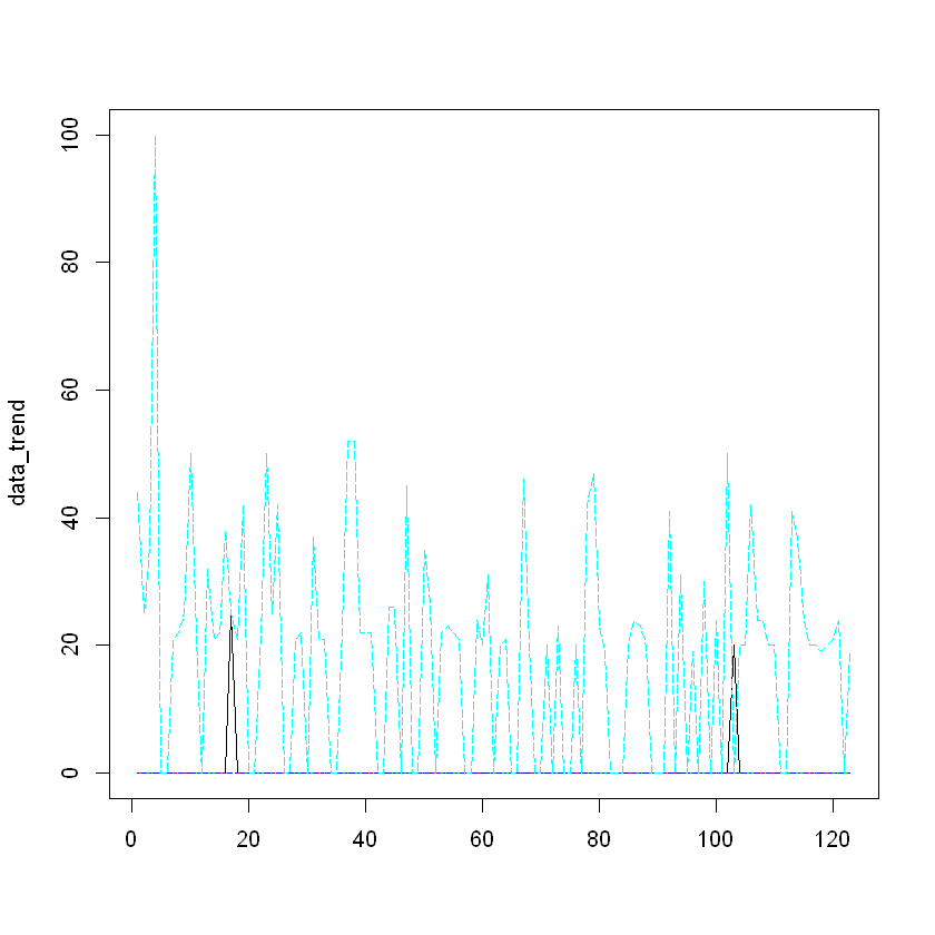
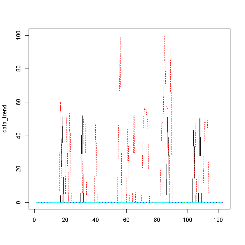
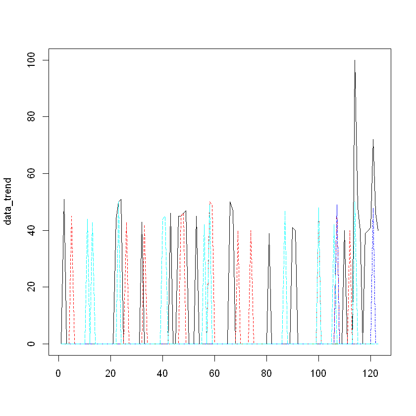
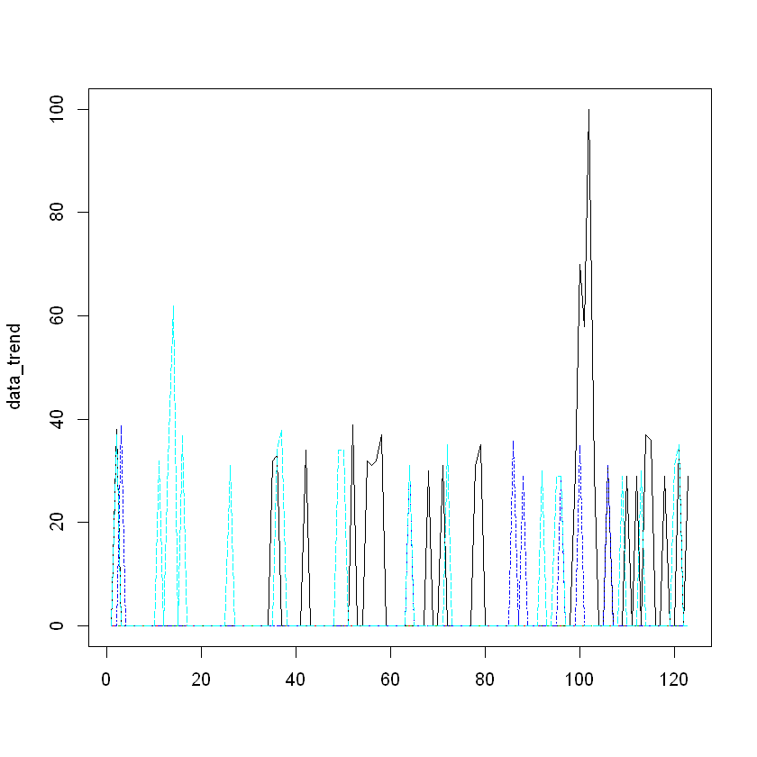
matplot(data_trend, type = "l")
<dl class=dl-horizontal> <dt>Day</dt> <dd>‘character’</dd> <dt>X12Degree.Brewing</dt> <dd>‘integer’</dd> <dt>Oskar.Blues.Grill…Brew</dt> <dd>‘integer’</dd> <dt>Whistle.Pig.Brewing.Company</dt> <dd>‘integer’</dd> <dt>Brix.Taphouse.and.Brewery</dt> <dd>‘integer’</dd> <dt>Moonlight.Pizza</dt> <dd>‘integer’</dd> </dl>
<dl class=dl-horizontal> <dt>Day</dt> <dd>‘character’</dd> <dt>X12Degree.Brewing</dt> <dd>‘integer’</dd> <dt>Oskar.Blues.Grill…Brew</dt> <dd>‘integer’</dd> <dt>Whistle.Pig.Brewing.Company</dt> <dd>‘integer’</dd> <dt>Brix.Taphouse.and.Brewery</dt> <dd>‘integer’</dd> <dt>Moonlight.Pizza</dt> <dd>‘integer’</dd> </dl>
<ol class=list-inline> <li>‘Day’</li> <li>‘X12Degree.Brewing’</li> <li>‘Oskar.Blues.Grill…Brew’</li> <li>‘Whistle.Pig.Brewing.Company’</li> <li>‘Brix.Taphouse.and.Brewery’</li> <li>‘Moonlight.Pizza’</li> </ol>
| Day | X12Degree.Brewing | Oskar.Blues.Grill...Brew | Whistle.Pig.Brewing.Company | Brix.Taphouse.and.Brewery | Moonlight.Pizza |
|---|---|---|---|---|---|
| 2016-07-01 | 0 | 0 | 0 | 0 | 44 |
| 2016-07-02 | 0 | 0 | 0 | 0 | 25 |
| 2016-07-03 | 0 | 0 | 0 | 0 | 35 |
| 2016-07-04 | 0 | 0 | 0 | 0 | 100 |
| 2016-07-05 | 0 | 0 | 0 | 0 | 0 |
| 2016-07-06 | 0 | 0 | 0 | 0 | 0 |
           y x1 x2 x3  x4
2016-07-01 0  0  0  0  44
2016-07-02 0  0  0  0  25
2016-07-03 0  0  0  0  35
2016-07-04 0  0  0  0 100
2016-07-05 0  0  0  0   0
2016-07-06 0  0  0  0   0
pre.period <- as.Date(c("2016-07-01", "2016-10-05"))
post.period <- as.Date(c("2016-10-09", "2016-10-31"))
impact <- CausalImpact(data_trend, pre.period, post.period)
################
options(warn=-1) # suppresses warnings form geom_path about missing row values
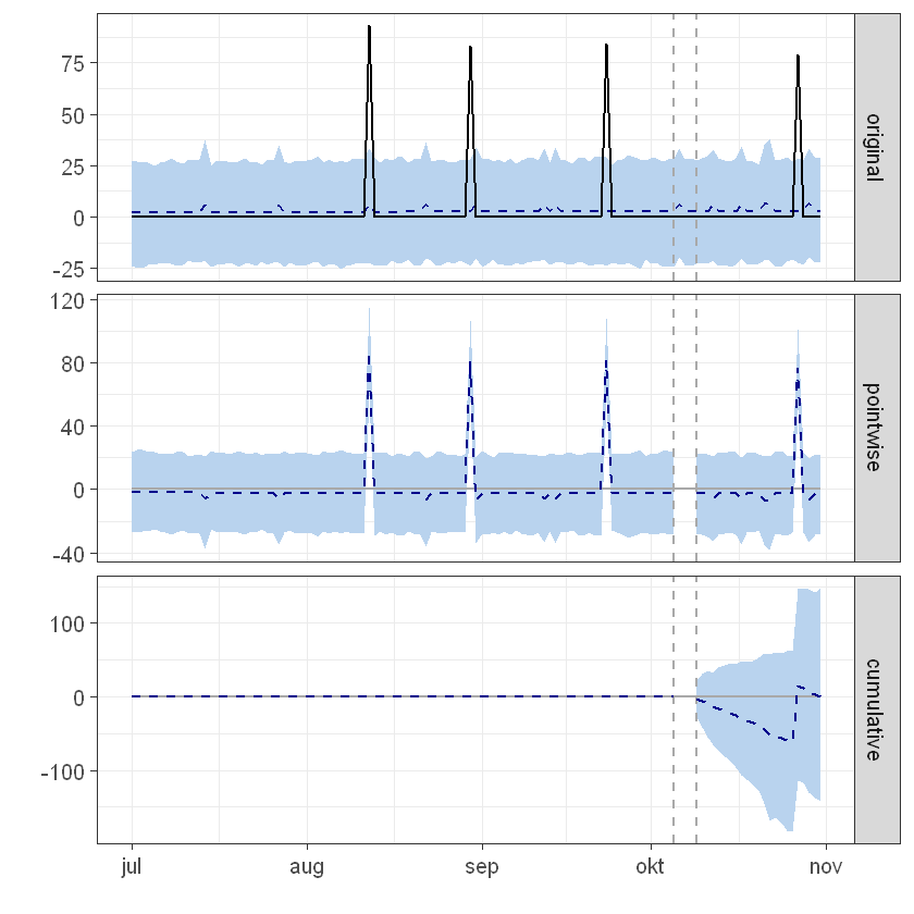
plot(impact)
options(warn=0) # restore warnings
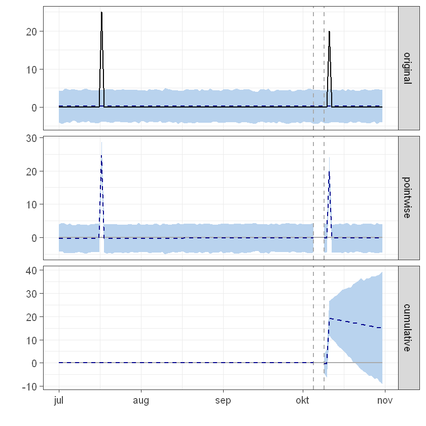
summary: 12Degree
summary(impact)

summary(impact,"report")

impact$summary
Posterior inference {CausalImpact}
Average Cumulative
Actual 0.87 20.00
Prediction (s.d.) 0.22 (0.55) 4.98 (12.56)
95% CI [-0.84, 1.3] [-19.36, 29.0]
Absolute effect (s.d.) 0.65 (0.55) 15.02 (12.56)
95% CI [-0.39, 1.7] [-9.04, 39.4]
Relative effect (s.d.) 302% (252%) 302% (252%)
95% CI [-182%, 791%] [-182%, 791%]
Posterior tail-area probability p: 0.118
Posterior prob. of a causal effect: 88%
For more details, type: summary(impact, "report")
Analysis report {CausalImpact}
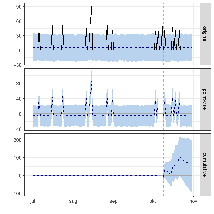
During the post-intervention period, the response variable had an average value of approx. 0.87. In the absence of an intervention, we would have expected an average response of 0.22. The 95% interval of this counterfactual prediction is [-0.84, 1.26]. Subtracting this prediction from the observed response yields an estimate of the causal effect the intervention had on the response variable. This effect is 0.65 with a 95% interval of [-0.39, 1.71]. For a discussion of the significance of this effect, see below.
Summing up the individual data points during the post-intervention period (which can only sometimes be meaningfully interpreted), the response variable had an overall value of 20.00. Had the intervention not taken place, we would have expected a sum of 4.98. The 95% interval of this prediction is [-19.36, 29.04].
The above results are given in terms of absolute numbers. In relative terms, the response variable showed an increase of +302%. The 95% interval of this percentage is [-182%, +791%].
This means that, although the intervention appears to have caused a positive effect, this effect is not statistically significant when considering the entire post-intervention period as a whole. Individual days or shorter stretches within the intervention period may of course still have had a significant effect, as indicated whenever the lower limit of the impact time series (lower plot) was above zero. The apparent effect could be the result of random fluctuations that are unrelated to the intervention. This is often the case when the intervention period is very long and includes much of the time when the effect has already worn off. It can also be the case when the intervention period is too short to distinguish the signal from the noise. Finally, failing to find a significant effect can happen when there are not enough control variables or when these variables do not correlate well with the response variable during the learning period.
The probability of obtaining this effect by chance is p = 0.118. This means the effect may be spurious and would generally not be considered statistically significant.
| Actual | Pred | Pred.lower | Pred.upper | Pred.sd | AbsEffect | AbsEffect.lower | AbsEffect.upper | AbsEffect.sd | RelEffect | RelEffect.lower | RelEffect.upper | RelEffect.sd | alpha | p | |
|---|---|---|---|---|---|---|---|---|---|---|---|---|---|---|---|
| Average | 0.8695652 | 0.216350 | -0.8417951 | 1.262463 | 0.5459336 | 0.6532152 | -0.3928982 | 1.71136 | 0.5459336 | 3.019252 | -1.81603 | 7.910146 | 2.523381 | 0.05 | 0.118 |
| Cumulative | 20.0000000 | 4.976051 | -19.3612875 | 29.036658 | 12.5564722 | 15.0239492 | -9.0366575 | 39.36129 | 12.5564722 | 3.019252 | -1.81603 | 7.910146 | 2.523381 | 0.05 | 0.118 |
Logsdon
trend.logsdon <- read.csv('timelines_causalimpact/multiTimeline (66).csv', sep = ',',
                        stringsAsFactors = FALSE)

sapply(trend.logsdon, typeof)
sapply(trend.logsdon, class)

colnames(trend.logsdon)
head(trend.logsdon)

################

y_trend <- trend.logsdon[2]
x1_trend <- trend.logsdon[3]
x2_trend <- trend.logsdon[4]
x3_trend <- trend.logsdon[5]
x4_trend <- trend.logsdon[6]


time.points <- seq.Date(as.Date("2016-07-01"), by = 1, length.out = nrow(y_trend))
data_trend <- zoo(cbind(y_trend, x1_trend, x2_trend, x3_trend, x4_trend), time.points)
colnames(data_trend) <- c("y", "x1", "x2", "x3", "x4")
head(data_trend)

matplot(data_trend, type = "l")

################

pre.period <- as.Date(c("2016-07-01", "2016-10-05"))
post.period <- as.Date(c("2016-10-09", "2016-10-31"))

impact <- CausalImpact(data_trend, pre.period, post.period)

options(warn=-1) # suppresses warnings form geom_path about missing row values
plot(impact)
options(warn=0)  # restore warnings

################

summary(impact)

summary(impact,"report")

impact$summary
<dl class=dl-horizontal> <dt>Day</dt> <dd>‘character’</dd> <dt>logsdon.farmhouse.ales</dt> <dd>‘integer’</dd> <dt>mazama.brewing</dt> <dd>‘integer’</dd> <dt>siuslaw.brewing</dt> <dd>‘integer’</dd> <dt>krauskis.brewskis</dt> <dd>‘integer’</dd> <dt>red.ox.brewing</dt> <dd>‘integer’</dd> </dl>
<dl class=dl-horizontal> <dt>Day</dt> <dd>‘character’</dd> <dt>logsdon.farmhouse.ales</dt> <dd>‘integer’</dd> <dt>mazama.brewing</dt> <dd>‘integer’</dd> <dt>siuslaw.brewing</dt> <dd>‘integer’</dd> <dt>krauskis.brewskis</dt> <dd>‘integer’</dd> <dt>red.ox.brewing</dt> <dd>‘integer’</dd> </dl>
<ol class=list-inline> <li>‘Day’</li> <li>‘logsdon.farmhouse.ales’</li> <li>‘mazama.brewing’</li> <li>‘siuslaw.brewing’</li> <li>‘krauskis.brewskis’</li> <li>‘red.ox.brewing’</li> </ol>
| Day | logsdon.farmhouse.ales | mazama.brewing | siuslaw.brewing | krauskis.brewskis | red.ox.brewing |
|---|---|---|---|---|---|
| 2016-07-01 | 0 | 0 | 0 | 0 | 0 |
| 2016-07-02 | 0 | 0 | 0 | 0 | 0 |
| 2016-07-03 | 0 | 0 | 0 | 0 | 0 |
| 2016-07-04 | 0 | 0 | 0 | 0 | 0 |
| 2016-07-05 | 0 | 0 | 0 | 0 | 0 |
| 2016-07-06 | 0 | 0 | 0 | 0 | 0 |
           y x1 x2 x3 x4
2016-07-01 0  0  0  0  0
2016-07-02 0  0  0  0  0
2016-07-03 0  0  0  0  0
2016-07-04 0  0  0  0  0
2016-07-05 0  0  0  0  0
2016-07-06 0  0  0  0  0
Posterior inference {CausalImpact}

                         Average        Cumulative
Actual                   4.5            104.0
Prediction (s.d.)        1.7 (2)        39.1 (45)
95% CI                   [-2.2, 5.7]    [-51.1, 130.3]

Absolute effect (s.d.)   2.8 (2)        64.9 (45)
95% CI                   [-1.1, 6.7]    [-26.3, 155.1]

Relative effect (s.d.)   166% (116%)    166% (116%)
95% CI                   [-67%, 397%]   [-67%, 397%]

Posterior tail-area probability p:   0.076
Posterior prob. of a causal effect:  92%

For more details, type: summary(impact, "report")

Analysis report {CausalImpact}


During the post-intervention period, the response variable had an average value of approx. 4.52. In the absence of an intervention, we would have expected an average response of 1.70. The 95% interval of this counterfactual prediction is [-2.22, 5.67]. Subtracting this prediction from the observed response yields an estimate of the causal effect the intervention had on the response variable. This effect is 2.82 with a 95% interval of [-1.14, 6.74]. For a discussion of the significance of this effect, see below.

Summing up the individual data points during the post-intervention period (which can only sometimes be meaningfully interpreted), the response variable had an overall value of 104.00. Had the intervention not taken place, we would have expected a sum of 39.07. The 95% interval of this prediction is [-51.12, 130.30].

The above results are given in terms of absolute numbers. In relative terms, the response variable showed an increase of +166%. The 95% interval of this percentage is [-67%, +397%].

This means that, although the intervention appears to have caused a positive effect, this effect is not statistically significant when considering the entire post-intervention period as a whole. Individual days or shorter stretches within the intervention period may of course still have had a significant effect, as indicated whenever the lower limit of the impact time series (lower plot) was above zero. The apparent effect could be the result of random fluctuations that are unrelated to the intervention. This is often the case when the intervention period is very long and includes much of the time when the effect has already worn off. It can also be the case when the intervention period is too short to distinguish the signal from the noise. Finally, failing to find a significant effect can happen when there are not enough control variables or when these variables do not correlate well with the response variable during the learning period.

The probability of obtaining this effect by chance is p = 0.076. This means the effect may be spurious and would generally not be considered statistically significant.
| Actual | Pred | Pred.lower | Pred.upper | Pred.sd | AbsEffect | AbsEffect.lower | AbsEffect.upper | AbsEffect.sd | RelEffect | RelEffect.lower | RelEffect.upper | RelEffect.sd | alpha | p | |
|---|---|---|---|---|---|---|---|---|---|---|---|---|---|---|---|
| Average | 4.521739 | 1.698626 | -2.222487 | 5.665054 | 1.97204 | 2.823113 | -1.143315 | 6.744226 | 1.97204 | 1.661997 | -0.6730822 | 3.9704 | 1.160962 | 0.05 | 0.076 |
| Cumulative | 104.000000 | 39.068408 | -51.117209 | 130.296251 | 45.35693 | 64.931592 | -26.296251 | 155.117209 | 45.35693 | 1.661997 | -0.6730822 | 3.9704 | 1.160962 | 0.05 | 0.076 |
Georgetown
trend.gt <- read.csv('timelines_causalimpact/multiTimeline (67).csv', sep = ',',
stringsAsFactors = FALSE)
sapply(trend.gt, typeof)
sapply(trend.gt, class)
colnames(trend.gt)
head(trend.gt)
################
y_trend <- trend.gt[2]
x1_trend <- trend.gt[3]
x2_trend <- trend.gt[4]
x3_trend <- trend.gt[5]
x4_trend <- trend.gt[6]
time.points <- seq.Date(as.Date("2016-07-01"), by = 1, length.out = nrow(y_trend))
data_trend <- zoo(cbind(y_trend, x1_trend, x2_trend, x3_trend, x4_trend), time.points)
colnames(data_trend) <- c("y", "x1", "x2", "x3", "x4")
head(data_trend)
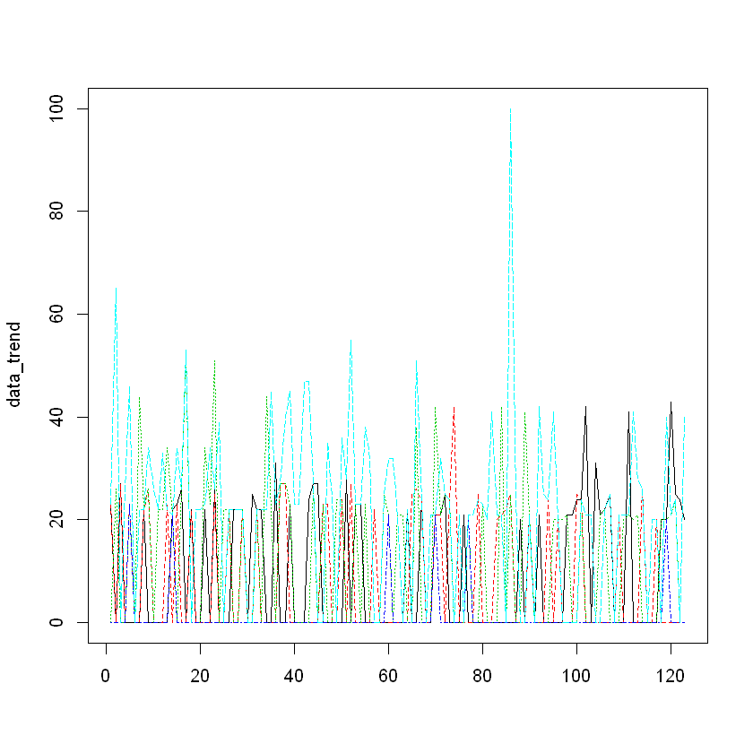
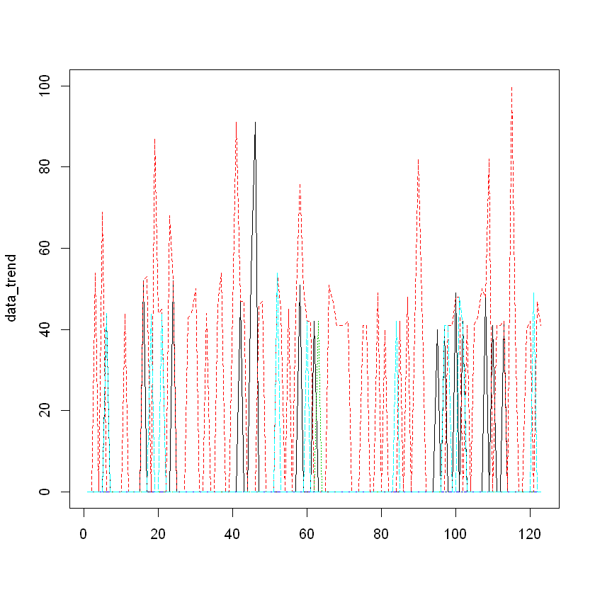
matplot(data_trend, type = "l")
################
pre.period <- as.Date(c("2016-07-01", "2016-10-05"))
post.period <- as.Date(c("2016-10-09", "2016-10-31"))
impact <- CausalImpact(data_trend, pre.period, post.period)
options(warn=-1) # suppresses warnings form geom_path about missing row values
plot(impact)
options(warn=0) # restore warnings
################
summary(impact)
summary(impact,"report")
impact$summary
<dl class=dl-horizontal> <dt>Day</dt> <dd>‘character’</dd> <dt>georgetown.brewing</dt> <dd>‘integer’</dd> <dt>fremont.brewing.company</dt> <dd>‘integer’</dd> <dt>redhook.brewery</dt> <dd>‘integer’</dd> <dt>mac.and.jacks.brewery</dt> <dd>‘integer’</dd> <dt>iron.horse.brewery</dt> <dd>‘integer’</dd> </dl>
<dl class=dl-horizontal> <dt>Day</dt> <dd>‘character’</dd> <dt>georgetown.brewing</dt> <dd>‘integer’</dd> <dt>fremont.brewing.company</dt> <dd>‘integer’</dd> <dt>redhook.brewery</dt> <dd>‘integer’</dd> <dt>mac.and.jacks.brewery</dt> <dd>‘integer’</dd> <dt>iron.horse.brewery</dt> <dd>‘integer’</dd> </dl>
<ol class=list-inline> <li>‘Day’</li> <li>‘georgetown.brewing’</li> <li>‘fremont.brewing.company’</li> <li>‘redhook.brewery’</li> <li>‘mac.and.jacks.brewery’</li> <li>‘iron.horse.brewery’</li> </ol>
| Day | georgetown.brewing | fremont.brewing.company | redhook.brewery | mac.and.jacks.brewery | iron.horse.brewery |
|---|---|---|---|---|---|
| 2016-07-01 | 23 | 23 | 0 | 0 | 23 |
| 2016-07-02 | 0 | 0 | 26 | 0 | 65 |
| 2016-07-03 | 27 | 27 | 0 | 0 | 0 |
| 2016-07-04 | 0 | 0 | 0 | 0 | 26 |
| 2016-07-05 | 0 | 23 | 23 | 23 | 46 |
| 2016-07-06 | 0 | 0 | 0 | 0 | 0 |
            y x1 x2 x3 x4
2016-07-01 23 23  0  0 23
2016-07-02  0  0 26  0 65
2016-07-03 27 27  0  0  0
2016-07-04  0  0  0  0 26
2016-07-05  0 23 23 23 46
2016-07-06  0  0  0  0  0
Posterior inference {CausalImpact}
Average Cumulative
Actual 16 358
Prediction (s.d.) 7.4 (2.4) 171.0 (54.3)
95% CI [3.1, 12] [71.3, 285]
Absolute effect (s.d.) 8.1 (2.4) 187.0 (54.3)
95% CI [3.2, 12] [73.2, 287]
Relative effect (s.d.) 109% (32%) 109% (32%)
95% CI [43%, 168%] [43%, 168%]
Posterior tail-area probability p: 0.001
Posterior prob. of a causal effect: 99.9%
For more details, type: summary(impact, "report")
Analysis report {CausalImpact}
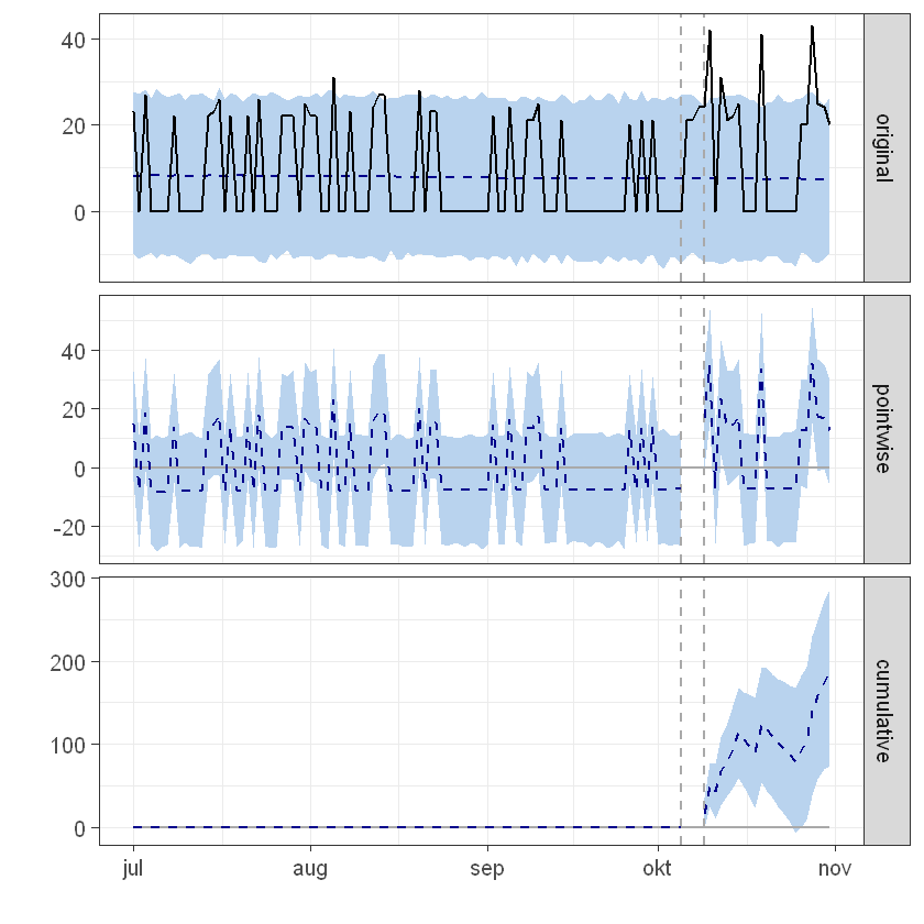
During the post-intervention period, the response variable had an average value of approx. 15.57. By contrast, in the absence of an intervention, we would have expected an average response of 7.44. The 95% interval of this counterfactual prediction is [3.10, 12.38]. Subtracting this prediction from the observed response yields an estimate of the causal effect the intervention had on the response variable. This effect is 8.13 with a 95% interval of [3.18, 12.46]. For a discussion of the significance of this effect, see below.
Summing up the individual data points during the post-intervention period (which can only sometimes be meaningfully interpreted), the response variable had an overall value of 358.00. By contrast, had the intervention not taken place, we would have expected a sum of 171.04. The 95% interval of this prediction is [71.33, 284.79].
The above results are given in terms of absolute numbers. In relative terms, the response variable showed an increase of +109%. The 95% interval of this percentage is [+43%, +168%].
This means that the positive effect observed during the intervention period is statistically significant and unlikely to be due to random fluctuations. It should be noted, however, that the question of whether this increase also bears substantive significance can only be answered by comparing the absolute effect (8.13) to the original goal of the underlying intervention.
The probability of obtaining this effect by chance is very small (Bayesian one-sided tail-area probability p = 0.001). This means the causal effect can be considered statistically significant.
| Actual | Pred | Pred.lower | Pred.upper | Pred.sd | AbsEffect | AbsEffect.lower | AbsEffect.upper | AbsEffect.sd | RelEffect | RelEffect.lower | RelEffect.upper | RelEffect.sd | alpha | p | |
|---|---|---|---|---|---|---|---|---|---|---|---|---|---|---|---|
| Average | 15.56522 | 7.436328 | 3.10136 | 12.38198 | 2.362591 | 8.12889 | 3.183239 | 12.46386 | 2.362591 | 1.093132 | 0.4280659 | 1.676077 | 0.3177093 | 0.05 | 0.001 |
| Cumulative | 358.00000 | 171.035537 | 71.33128 | 284.78551 | 54.339583 | 186.96446 | 73.214486 | 286.66872 | 54.339583 | 1.093132 | 0.4280659 | 1.676077 | 0.3177093 | 0.05 | 0.001 |
Uberbrew
trend.ub <- read.csv('timelines_causalimpact/multiTimeline (68).csv', sep = ',',
                        stringsAsFactors = FALSE)

sapply(trend.ub, typeof)
sapply(trend.ub, class)

colnames(trend.ub)
head(trend.ub)

################

y_trend <- trend.ub[2]
x1_trend <- trend.ub[3]
x2_trend <- trend.ub[4]
x3_trend <- trend.ub[5]
x4_trend <- trend.ub[6]


time.points <- seq.Date(as.Date("2016-07-01"), by = 1, length.out = nrow(y_trend))
data_trend <- zoo(cbind(y_trend, x1_trend, x2_trend, x3_trend, x4_trend), time.points)
colnames(data_trend) <- c("y", "x1", "x2", "x3", "x4")
head(data_trend)

matplot(data_trend, type = "l")

################

pre.period <- as.Date(c("2016-07-01", "2016-10-05"))
post.period <- as.Date(c("2016-10-09", "2016-10-31"))

impact <- CausalImpact(data_trend, pre.period, post.period)

options(warn=-1) # suppresses warnings form geom_path about missing row values
plot(impact)
options(warn=0)  # restore warnings

################

summary(impact)

summary(impact,"report")

impact$summary
<dl class=dl-horizontal> <dt>Day</dt> <dd>‘character’</dd> <dt>uberbrew</dt> <dd>‘integer’</dd> <dt>bridger.brewing</dt> <dd>‘integer’</dd> <dt>cabinet.mountain.brewing</dt> <dd>‘integer’</dd> <dt>the.front.brewing.company</dt> <dd>‘integer’</dd> <dt>backslope.brewing</dt> <dd>‘integer’</dd> </dl>
<dl class=dl-horizontal> <dt>Day</dt> <dd>‘character’</dd> <dt>uberbrew</dt> <dd>‘integer’</dd> <dt>bridger.brewing</dt> <dd>‘integer’</dd> <dt>cabinet.mountain.brewing</dt> <dd>‘integer’</dd> <dt>the.front.brewing.company</dt> <dd>‘integer’</dd> <dt>backslope.brewing</dt> <dd>‘integer’</dd> </dl>
<ol class=list-inline> <li>‘Day’</li> <li>‘uberbrew’</li> <li>‘bridger.brewing’</li> <li>‘cabinet.mountain.brewing’</li> <li>‘the.front.brewing.company’</li> <li>‘backslope.brewing’</li> </ol>
| Day | uberbrew | bridger.brewing | cabinet.mountain.brewing | the.front.brewing.company | backslope.brewing |
|---|---|---|---|---|---|
| 2016-07-01 | 0 | 0 | 0 | 0 | 0 |
| 2016-07-02 | 0 | 0 | 0 | 0 | 0 |
| 2016-07-03 | 0 | 54 | 0 | 0 | 0 |
| 2016-07-04 | 0 | 0 | 0 | 0 | 0 |
| 2016-07-05 | 0 | 69 | 0 | 0 | 0 |
| 2016-07-06 | 44 | 0 | 0 | 0 | 44 |
            y x1 x2 x3 x4
2016-07-01  0  0  0  0  0
2016-07-02  0  0  0  0  0
2016-07-03  0 54  0  0  0
2016-07-04  0  0  0  0  0
2016-07-05  0 69  0  0  0
2016-07-06 44  0  0  0 44
Posterior inference {CausalImpact}

                         Average        Cumulative
Actual                   7.5            173.0
Prediction (s.d.)        5.3 (3.4)      120.8 (77.5)
95% CI                   [-1.2, 12]     [-27.3, 271]

Absolute effect (s.d.)   2.3 (3.4)      52.2 (77.5)
95% CI                   [-4.3, 8.7]    [-98.3, 200.3]

Relative effect (s.d.)   43% (64%)      43% (64%)
95% CI                   [-81%, 166%]   [-81%, 166%]

Posterior tail-area probability p:   0.244
Posterior prob. of a causal effect:  76%

For more details, type: summary(impact, "report")

Analysis report {CausalImpact}


During the post-intervention period, the response variable had an average value of approx. 7.52. In the absence of an intervention, we would have expected an average response of 5.25. The 95% interval of this counterfactual prediction is [-1.19, 11.80]. Subtracting this prediction from the observed response yields an estimate of the causal effect the intervention had on the response variable. This effect is 2.27 with a 95% interval of [-4.27, 8.71]. For a discussion of the significance of this effect, see below.

Summing up the individual data points during the post-intervention period (which can only sometimes be meaningfully interpreted), the response variable had an overall value of 173.00. Had the intervention not taken place, we would have expected a sum of 120.77. The 95% interval of this prediction is [-27.27, 271.31].

The above results are given in terms of absolute numbers. In relative terms, the response variable showed an increase of +43%. The 95% interval of this percentage is [-81%, +166%].

This means that, although the intervention appears to have caused a positive effect, this effect is not statistically significant when considering the entire post-intervention period as a whole. Individual days or shorter stretches within the intervention period may of course still have had a significant effect, as indicated whenever the lower limit of the impact time series (lower plot) was above zero. The apparent effect could be the result of random fluctuations that are unrelated to the intervention. This is often the case when the intervention period is very long and includes much of the time when the effect has already worn off. It can also be the case when the intervention period is too short to distinguish the signal from the noise. Finally, failing to find a significant effect can happen when there are not enough control variables or when these variables do not correlate well with the response variable during the learning period.

The probability of obtaining this effect by chance is p = 0.244. This means the effect may be spurious and would generally not be considered statistically significant.
| Actual | Pred | Pred.lower | Pred.upper | Pred.sd | AbsEffect | AbsEffect.lower | AbsEffect.upper | AbsEffect.sd | RelEffect | RelEffect.lower | RelEffect.upper | RelEffect.sd | alpha | p | |
|---|---|---|---|---|---|---|---|---|---|---|---|---|---|---|---|
| Average | 7.521739 | 5.250878 | -1.185505 | 11.7962 | 3.371324 | 2.270861 | -4.274465 | 8.707244 | 3.371324 | 0.4324726 | -0.8140475 | 1.658245 | 0.6420496 | 0.05 | 0.244 |
| Cumulative | 173.000000 | 120.770202 | -27.266613 | 271.3127 | 77.540462 | 52.229798 | -98.312685 | 200.266613 | 77.540462 | 0.4324726 | -0.8140475 | 1.658245 | 0.6420496 | 0.05 | 0.244 |
Hardywood
trend.hardy <- read.csv('timelines_causalimpact/multiTimeline (69).csv', sep = ',',
stringsAsFactors = FALSE)
sapply(trend.hardy, typeof)
sapply(trend.hardy, class)
colnames(trend.hardy)
head(trend.hardy)
################
y_trend <- trend.hardy[2]
x1_trend <- trend.hardy[3]
x2_trend <- trend.hardy[4]
x3_trend <- trend.hardy[5]
x4_trend <- trend.hardy[6]
time.points <- seq.Date(as.Date("2016-07-01"), by = 1, length.out = nrow(y_trend))
data_trend <- zoo(cbind(y_trend, x1_trend, x2_trend, x3_trend, x4_trend), time.points)
colnames(data_trend) <- c("y", "x1", "x2", "x3", "x4")
head(data_trend)
matplot(data_trend, type = "l")
################
pre.period <- as.Date(c("2016-07-01", "2016-10-05"))
post.period <- as.Date(c("2016-10-09", "2016-10-31"))
impact <- CausalImpact(data_trend, pre.period, post.period)
options(warn=-1) # suppresses warnings form geom_path about missing row values
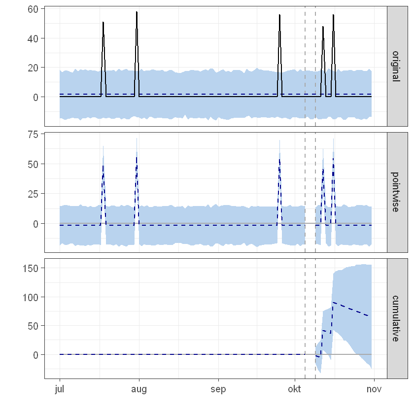
plot(impact)
options(warn=0) # restore warnings
################
summary(impact)
summary(impact,"report")
impact$summary
<dl class=dl-horizontal> <dt>Day</dt> <dd>‘character’</dd> <dt>hardywood.park.craft.brewery</dt> <dd>‘integer’</dd> <dt>lickinghole.creek.craft.brewery</dt> <dd>‘integer’</dd> <dt>barrel.oak.farm.taphouse</dt> <dd>‘integer’</dd> <dt>sunken.city.brewing.company</dt> <dd>‘integer’</dd> <dt>new.district.brewing.company</dt> <dd>‘integer’</dd> </dl>
<dl class=dl-horizontal> <dt>Day</dt> <dd>‘character’</dd> <dt>hardywood.park.craft.brewery</dt> <dd>‘integer’</dd> <dt>lickinghole.creek.craft.brewery</dt> <dd>‘integer’</dd> <dt>barrel.oak.farm.taphouse</dt> <dd>‘integer’</dd> <dt>sunken.city.brewing.company</dt> <dd>‘integer’</dd> <dt>new.district.brewing.company</dt> <dd>‘integer’</dd> </dl>
<ol class=list-inline> <li>‘Day’</li> <li>‘hardywood.park.craft.brewery’</li> <li>‘lickinghole.creek.craft.brewery’</li> <li>‘barrel.oak.farm.taphouse’</li> <li>‘sunken.city.brewing.company’</li> <li>‘new.district.brewing.company’</li> </ol>
| Day | hardywood.park.craft.brewery | lickinghole.creek.craft.brewery | barrel.oak.farm.taphouse | sunken.city.brewing.company | new.district.brewing.company |
|---|---|---|---|---|---|
| 2016-07-01 | 0 | 0 | 0 | 0 | 0 |
| 2016-07-02 | 51 | 0 | 0 | 0 | 0 |
| 2016-07-03 | 0 | 0 | 0 | 0 | 0 |
| 2016-07-04 | 0 | 0 | 0 | 0 | 0 |
| 2016-07-05 | 0 | 45 | 0 | 0 | 0 |
| 2016-07-06 | 0 | 0 | 0 | 0 | 0 |
            y x1 x2 x3 x4
2016-07-01  0  0  0  0  0
2016-07-02 51  0  0  0  0
2016-07-03  0  0  0  0  0
2016-07-04  0  0  0  0  0
2016-07-05  0 45  0  0  0
2016-07-06  0  0  0  0  0
Posterior inference {CausalImpact}

                         Average            Cumulative
Actual                   22                 506
Prediction (s.d.)        2 (78)             46 (1801)
95% CI                   [-179, 169]        [-4116, 3893]

Absolute effect (s.d.)   20 (78)            460 (1801)
95% CI                   [-147, 201]        [-3387, 4622]

Relative effect (s.d.)   1001% (3919%)      1001% (3919%)
95% CI                   [-7371%, 10059%]   [-7371%, 10059%]

Posterior tail-area probability p:   0.24358
Posterior prob. of a causal effect:  76%

For more details, type: summary(impact, "report")

Analysis report {CausalImpact}


During the post-intervention period, the response variable had an average value of approx. 22.00. In the absence of an intervention, we would have expected an average response of 2.00. The 95% interval of this counterfactual prediction is [-178.97, 169.27]. Subtracting this prediction from the observed response yields an estimate of the causal effect the intervention had on the response variable. This effect is 20.00 with a 95% interval of [-147.27, 200.97]. For a discussion of the significance of this effect, see below.

Summing up the individual data points during the post-intervention period (which can only sometimes be meaningfully interpreted), the response variable had an overall value of 506.00. Had the intervention not taken place, we would have expected a sum of 45.95. The 95% interval of this prediction is [-4116.24, 3893.30].

The above results are given in terms of absolute numbers. In relative terms, the response variable showed an increase of +1001%. The 95% interval of this percentage is [-7371%, +10059%].

This means that, although the intervention appears to have caused a positive effect, this effect is not statistically significant when considering the entire post-intervention period as a whole. Individual days or shorter stretches within the intervention period may of course still have had a significant effect, as indicated whenever the lower limit of the impact time series (lower plot) was above zero. The apparent effect could be the result of random fluctuations that are unrelated to the intervention. This is often the case when the intervention period is very long and includes much of the time when the effect has already worn off. It can also be the case when the intervention period is too short to distinguish the signal from the noise. Finally, failing to find a significant effect can happen when there are not enough control variables or when these variables do not correlate well with the response variable during the learning period.

The probability of obtaining this effect by chance is p = 0.244. This means the effect may be spurious and would generally not be considered statistically significant.
| Actual | Pred | Pred.lower | Pred.upper | Pred.sd | AbsEffect | AbsEffect.lower | AbsEffect.upper | AbsEffect.sd | RelEffect | RelEffect.lower | RelEffect.upper | RelEffect.sd | alpha | p | |
|---|---|---|---|---|---|---|---|---|---|---|---|---|---|---|---|
| Average | 22 | 1.997902 | -178.9668 | 169.2737 | 78.29663 | 20.0021 | -147.2737 | 200.9668 | 78.29663 | 10.01155 | -73.71419 | 100.5889 | 39.18942 | 0.05 | 0.2435766 |
| Cumulative | 506 | 45.951749 | -4116.2358 | 3893.2958 | 1800.82244 | 460.0483 | -3387.2958 | 4622.2358 | 1800.82244 | 10.01155 | -73.71419 | 100.5889 | 39.18942 | 0.05 | 0.2435766 |
Brown Truck
trend.browntruck <- read.csv('timelines_causalimpact/multiTimeline (70).csv', sep = ',',
                        stringsAsFactors = FALSE)

sapply(trend.browntruck, typeof)
sapply(trend.browntruck, class)

colnames(trend.browntruck)
head(trend.browntruck)

################

y_trend <- trend.browntruck[2]
x1_trend <- trend.browntruck[3]
x2_trend <- trend.browntruck[4]
x3_trend <- trend.browntruck[5]
x4_trend <- trend.browntruck[6]


time.points <- seq.Date(as.Date("2016-07-01"), by = 1, length.out = nrow(y_trend))
data_trend <- zoo(cbind(y_trend, x1_trend, x2_trend, x3_trend, x4_trend), time.points)
colnames(data_trend) <- c("y", "x1", "x2", "x3", "x4")
head(data_trend)

matplot(data_trend, type = "l")

################

pre.period <- as.Date(c("2016-07-01", "2016-10-05"))
post.period <- as.Date(c("2016-10-09", "2016-10-31"))

impact <- CausalImpact(data_trend, pre.period, post.period)

options(warn=-1) # suppresses warnings form geom_path about missing row values
plot(impact)
options(warn=0)  # restore warnings

################

summary(impact)

summary(impact,"report")

impact$summary
<dl class=dl-horizontal> <dt>Day</dt> <dd>‘character’</dd> <dt>brown.truck.brewery</dt> <dd>‘integer’</dd> <dt>good.hops.brewing.llc</dt> <dd>‘integer’</dd> <dt>preyer.brewing.company</dt> <dd>‘integer’</dd> <dt>fortnight.brewing.company</dt> <dd>‘integer’</dd> <dt>burial.beer.co</dt> <dd>‘integer’</dd> </dl>
<dl class=dl-horizontal> <dt>Day</dt> <dd>‘character’</dd> <dt>brown.truck.brewery</dt> <dd>‘integer’</dd> <dt>good.hops.brewing.llc</dt> <dd>‘integer’</dd> <dt>preyer.brewing.company</dt> <dd>‘integer’</dd> <dt>fortnight.brewing.company</dt> <dd>‘integer’</dd> <dt>burial.beer.co</dt> <dd>‘integer’</dd> </dl>
<ol class=list-inline> <li>‘Day’</li> <li>‘brown.truck.brewery’</li> <li>‘good.hops.brewing.llc’</li> <li>‘preyer.brewing.company’</li> <li>‘fortnight.brewing.company’</li> <li>‘burial.beer.co’</li> </ol>
| Day | brown.truck.brewery | good.hops.brewing.llc | preyer.brewing.company | fortnight.brewing.company | burial.beer.co |
|---|---|---|---|---|---|
| 2016-07-01 | 0 | 0 | 0 | 0 | 0 |
| 2016-07-02 | 38 | 0 | 0 | 0 | 37 |
| 2016-07-03 | 0 | 0 | 0 | 39 | 0 |
| 2016-07-04 | 0 | 0 | 0 | 0 | 0 |
| 2016-07-05 | 0 | 0 | 0 | 0 | 0 |
| 2016-07-06 | 0 | 0 | 0 | 0 | 0 |
            y x1 x2 x3 x4
2016-07-01  0  0  0  0  0
2016-07-02 38  0  0  0 37
2016-07-03  0  0  0 39  0
2016-07-04  0  0  0  0  0
2016-07-05  0  0  0  0  0
2016-07-06  0  0  0  0  0
Posterior inference {CausalImpact}

                         Average         Cumulative
Actual                   19              443
Prediction (s.d.)        4.5 (2.5)       103.3 (56.6)
95% CI                   [-0.026, 9.6]   [-0.600, 221.7]

Absolute effect (s.d.)   15 (2.5)        340 (56.6)
95% CI                   [9.6, 19]       [221.3, 444]

Relative effect (s.d.)   329% (55%)      329% (55%)
95% CI                   [214%, 430%]    [214%, 430%]

Posterior tail-area probability p:   0.001
Posterior prob. of a causal effect:  99.9%

For more details, type: summary(impact, "report")

Analysis report {CausalImpact}


During the post-intervention period, the response variable had an average value of approx. 19.26. By contrast, in the absence of an intervention, we would have expected an average response of 4.49. The 95% interval of this counterfactual prediction is [-0.026, 9.64]. Subtracting this prediction from the observed response yields an estimate of the causal effect the intervention had on the response variable. This effect is 14.77 with a 95% interval of [9.62, 19.29]. For a discussion of the significance of this effect, see below.

Summing up the individual data points during the post-intervention period (which can only sometimes be meaningfully interpreted), the response variable had an overall value of 443.00. By contrast, had the intervention not taken place, we would have expected a sum of 103.28. The 95% interval of this prediction is [-0.60, 221.65].

The above results are given in terms of absolute numbers. In relative terms, the response variable showed an increase of +329%. The 95% interval of this percentage is [+214%, +430%].

This means that the positive effect observed during the intervention period is statistically significant and unlikely to be due to random fluctuations. It should be noted, however, that the question of whether this increase also bears substantive significance can only be answered by comparing the absolute effect (14.77) to the original goal of the underlying intervention.

The probability of obtaining this effect by chance is very small (Bayesian one-sided tail-area probability p = 0.001). This means the causal effect can be considered statistically significant.
| Actual | Pred | Pred.lower | Pred.upper | Pred.sd | AbsEffect | AbsEffect.lower | AbsEffect.upper | AbsEffect.sd | RelEffect | RelEffect.lower | RelEffect.upper | RelEffect.sd | alpha | p | |
|---|---|---|---|---|---|---|---|---|---|---|---|---|---|---|---|
| Average | 19.26087 | 4.490307 | -0.02608773 | 9.637096 | 2.459114 | 14.77056 | 9.623774 | 19.28696 | 2.459114 | 3.289432 | 2.143233 | 4.295242 | 0.5476493 | 0.05 | 0.001 |
| Cumulative | 443.00000 | 103.277068 | -0.60001768 | 221.653197 | 56.559618 | 339.72293 | 221.346803 | 443.60002 | 56.559618 | 3.289432 | 2.143233 | 4.295242 | 0.5476493 | 0.05 | 0.001 |